
Neural Nets
Part 1 - Multi-Layer Perceptrons

Motivation
To reliably attack a technology well, we need to understand it on a deep level. This blog post is part of an effort to get a gears-level understanding of LLMs for the purposes of attacking them and their surrounding infrastructure. This will be part of a series of posts building up my current knowledge. I don’t yet know which topics I’ll be covering or in what order yet, we will see where the learning takes me!
This specific post is an introduction to Multi-Layer Perceptrons (MLPs), one of the simplest types of neural networks, yet still a core building block of the architecture that makes up LLMs. In this post, we will set up the purpose and structure of an MLP, and in the next post we will discuss what it means to actually “train” a model.
Beyond these first two posts, I plan to go into greater depth on the math behind MLPs, and we’ll also implement one in Python to solidify our comprehension.
Input Layers
We’ll use the canonical example of training a model to classify handwritten digits. In particular, given an image of a handwritten digit between 0 and 9, we want our model to correctly identify the correct digit.
Like any computer image, a digital copy of a hand-written digit will be made up entirely of pixels. For simplicity, we’ll assume a white background and black digits, with no greyscale gradients.
We’ll also normalize our pixel-grid so that all digits are written on the same size background. The textbook example is a 28 x 28 = 784 grid of pixels. That is what we’ll use here. Each pixel is given a value: 0 for white and 1 for black. Then we take the 2D matrix of values and flatten or reshape them into a 1D vector. This means that the total input we’ll provide to our network is 784 numbers, where each number is either 0 or 1.
Instead of writing our vector out in standard notation, we will represent each value by a node in a graph, referred to as a “neuron”, as follows. This column of nodes or neurons represents our 784 inputs. For legibility, this image only shows 20 neurons. Imagine that there are 784 of them, indicated by the “n = 784” text at the bottom of the column:

Output Layers
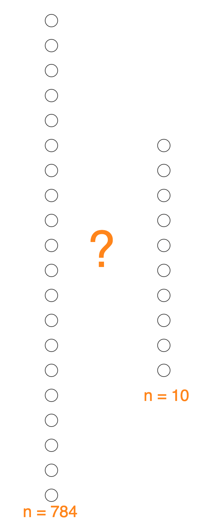
So far we’ve arranged our input into a column of 784 neurons, each of which holds either a 0 or 1. Recall, we want to give our model this set of values, and output the correct digit represented by the handwritten image. What we need is a very complex function that somehow takes in our 784 values, and outputs one of the the ten possible digits. Generally, this is what a neural network is: a function that takes in one set of numbers, and outputs another set of numbers.
Another way we can express this is to say that our input-space has 784 dimensions, and our output space has 10 dimensions. Each neuron in the output represents one of the ten digits. Somehow (represented by the big orange question mark), we need to get from our input to select a specific value in the output column. But instead of using the word “column”, we’ll refer to each dimensional space as a “layer” of our network:
Hidden Layers
It is possible to create a neural network with only two layers. This would be a single-layer perceptron. To make it an MLP, we would need at least one or more “hidden” layers. The more hidden layers we use, the more computational expressiveness we can get out of the network. In other words, the more interesting features of our dataset we can get the network to “understand”.
We’ll again use the textbook example, and create a network with only one hidden layer. Both the number of hidden layers and number of neurons per layer are somewhat arbitrary choices, and a future post might explore how we could go about choosing an appropriate value for these depending on the problem we’re trying to solve. For now, we’ll simply use one hidden layer of 100 neurons. Again, note that we’re only drawing 16 neurons for better readability:
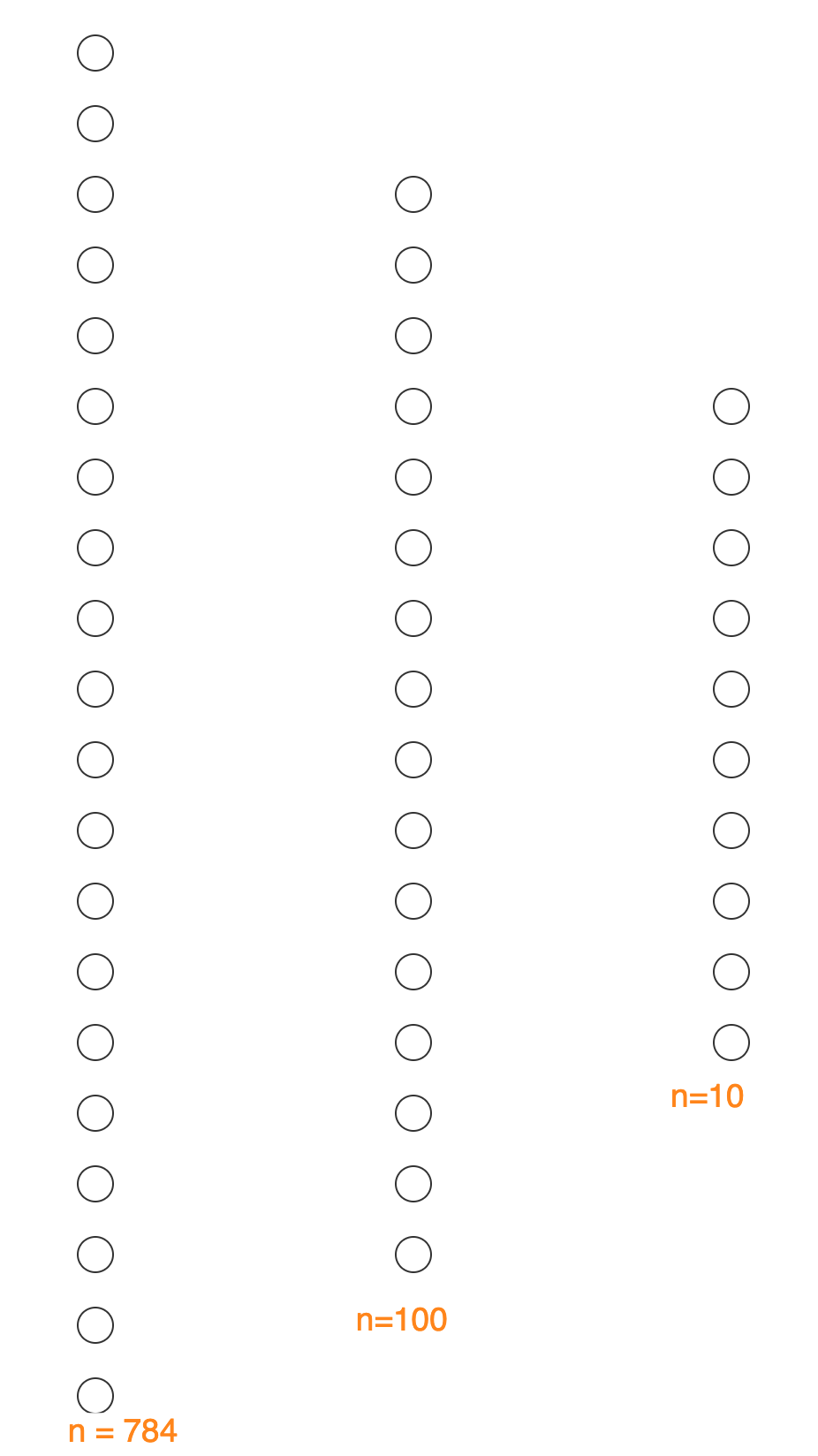
Neurons are the fundamental unit of any neural network. Our model has three kinds of neurons:
Input neurons are given initial values based on the data we want to feed to the network. In this case, our vector of zeros and ones representing a hand-written image. Input neurons always live in Layer 1 of N, where N is the total number of layers.
Hidden neurons make up any layers between the input and output neurons. But what values do these have, and how do they get them? Each neuron in layer L gets its input from all the neurons in layer L − 1 (in a fully-connected network). We’ll talk more about these connections and how they work below.
Output neurons comprise the final layer, and they get their input from all the neurons in the layer that precedes it, layer N- 1.
Parameters
To make this model a network, we need some way for the neurons to communicate information with each other. In an MLP, neurons only communicate forward. This means neurons in Layer L transmit information to neurons in Layer L + 1, and so on. MLPs are in fact known as a type of “feedforward” network for this reason. We can represent lines of communication via edges in our graph:
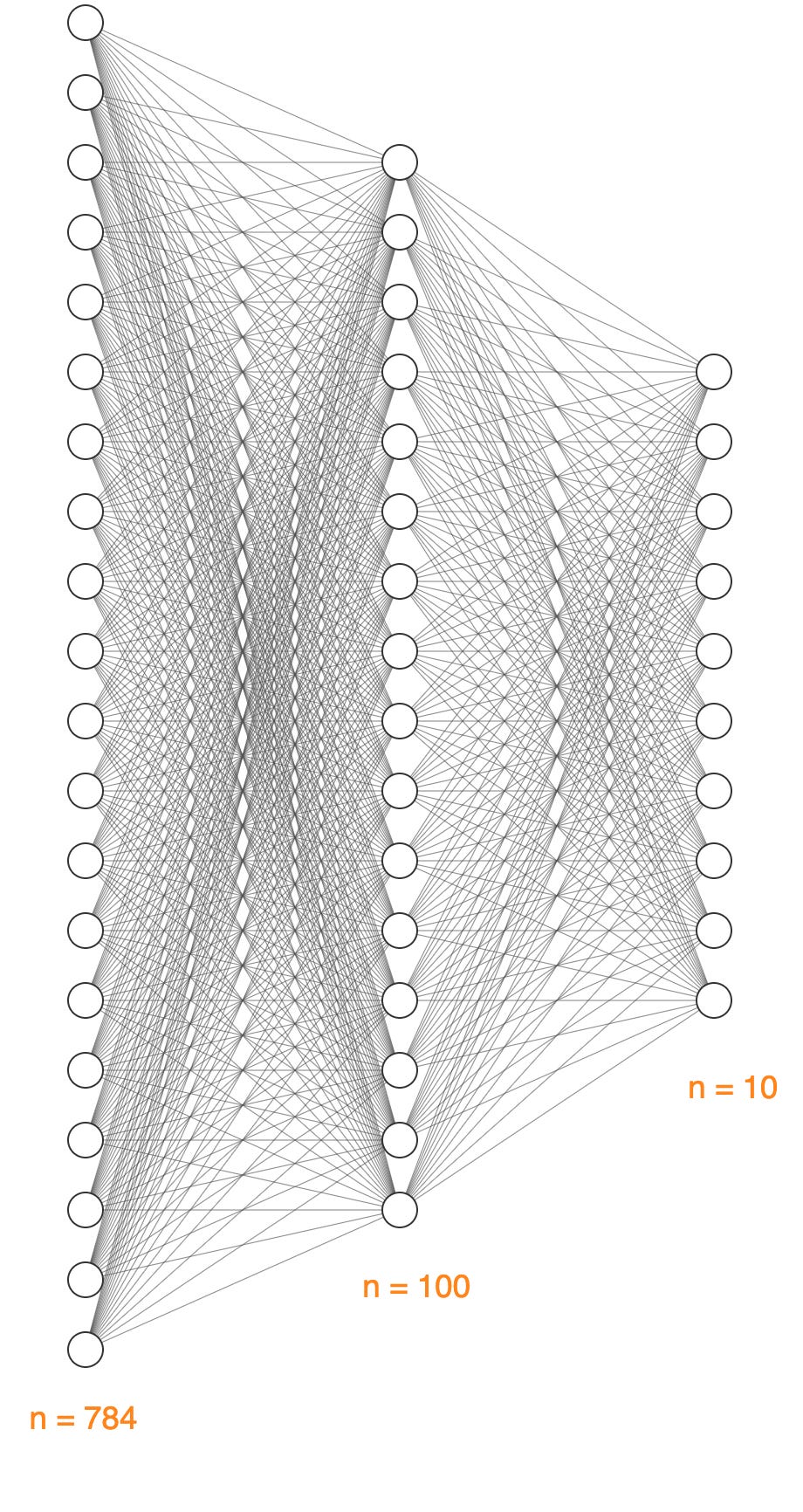
Remember that the image above isn’t to scale, so it contains significantly less connections that the actual model. In a fully connected MLP like the one we are building, the value of every neuron in Layer L influences the value of every neuron in Layer L + 1. To calculate the total number of connections between any two layers, we take the number of neurons in Layer L and multiply them by the number in Layer L + 1. Then we can sum up these products to determine the total number of connections for our network. In our case, that means (784 x 100) + (100 x 10) = 79,400 . This seems like a very big number, but bear in mind that modern LLMs have trillions of these connections! That’s what makes them Large.
Let’s recap: we have three layers of neurons, each of which holds a value. The neurons in the first layer hold a number representing the value of a particular pixel in a 28 x 28 grid. Each remaining neurons get a value that depends on the connections between itself and all the neurons that preceded it. Where do these values come from?
We can think about each connection between neurons as a “weight”: they tell us how strongly the two neurons are connected together. If a weight X between neuron A and neuron B is strong, then neuron A is going to have relatively high influence on the value of neuron B.
So a neuron’s value is almost fully determined by the value of all the neurons in the layer preceding it, and the value of all the weights connecting it to each preceding neuron. In particular, we can almost calculate the value of a neuron by taking the sum of all the neuron values times each weight of the preceding layer and passing it through a function that will decide its final value.
I say almost, because there is one more term that is going to influence our network, called a “bias”. Every neuron that lives in any layer beyond the first one gets a bias. A bias is a kind of friction coefficient: it tells us how susceptible that neuron is to influence from earlier neurons regardless of the weight. Each neuron beyond the input layer has its own bias, so there are 110 biases in total.
A small aside here, because this analogy helped things click for me. Remember how the equation of a line can be expressed as y = ax + b ? In this equation, a governs the slope of the line: it tells us how steep it is. And b determines the “y intercept”, the point where it begins on the Y axis. The line is fully determined by the values of a and b.
Similarly, our neural network is fully determined by the values of all the weights and all the biases. Weights are like a because they are a coefficient to a variable, whereas biases are like b because they are constant values. a and b are called “parameters”, and we use the same term in machine learning. The total number of parameters in our network is therefore 79,400 + 110 = 79,510 .
What’s Next?
The big question we have in front of us is, if the value of non-layer 1 neurons are determined by layer 1 neurons and the values of all parameters… where do the parameters get their values from?
The short answer to that question is, “training”. When we say that a model or a network “learns”, what we mean is that the weights acquire specific values that make our model become a reliable function for the problem we are trying to solve.
In the next post, we’ll provide a long answer to this question, and try to understand how a series of circles and lines can reliably read a handwritten digit.